I wanted to train a ~3.8B hybrid model for agentic and coding work, so I tested architecture changes on 60M and 200M models first. Four ideas came out of it. Three of them, plus two published methods, make up the model the report calls F: a 3:1 Gated DeltaNet (GDN)–attention hybrid. At 200M, F has 2.1% lower bits per byte than the base (two seeds each; the gap is far larger than the difference between seeds). Yes, 200M is small. At 60M, where I could train longer, the base needs about 1.5 times F’s training FLOPs to match it, with one seed per point. FLOPs aren’t wall-clock time, though: on my unfused code, block-entry mixing makes each step about 3% slower and the GDN mixes 13% to 18%. The fourth idea, grid KV sharing, came last and was tested separately. This post goes through where each idea came from and how far the evidence goes.
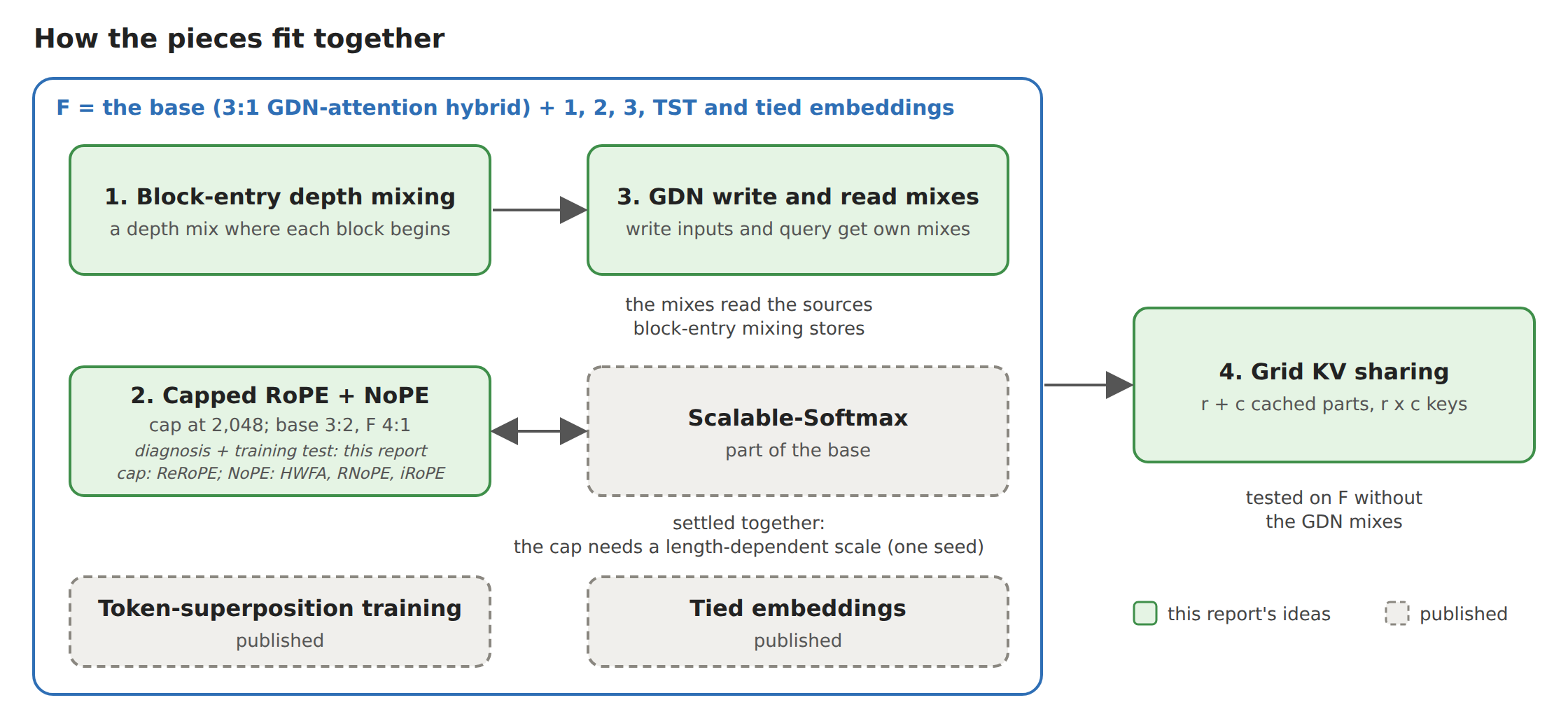
Ideas 1 to 3 and two published methods make up F. Idea 4 came last. I tested it on F without the GDN mixes.
Background
The compute for the full 3.8B run never came through, so the work stopped at the small-model stage.
Gated DeltaNet (GDN), from Songlin Yang, Jan Kautz and Ali Hatamizadeh, is a linear-attention layer with a fixed-size recurrent state. My hybrids have three GDN layers for every softmax-attention layer (3:1). The base is the same hybrid without block-entry mixing, the GDN mixes, token-superposition training (TST) and tied embeddings. It already uses the capped RoPE of idea 2, with two attention layers left without positions instead of one. Ideas 1, 2 and 4 build on published methods, which I name in their sections.
I watched two numbers the whole time: bits per byte (bpb) on held-out text, and retrieval far past the 8k training length. An agent has to find things in long logs and tool output, and the loss alone won’t tell you whether it can. Retrieval here means synthetic lookups: a long document hides one needle, or 4 or 16 key–value pairs, and the model must return the right value, scored by exact match.
The fourth idea, grid key–value (KV) sharing, keeps the cache and compute of grouped-query attention (GQA; Joshua Ainslie et al., 2023) but gives the heads more distinct keys. At 200M it matched GQA at the same cache, but fell behind with less cache: it changes how heads share the cache but doesn’t make up for a smaller one. Everything below is in the full report, with every table and caveat: the report PDF on GitHub.
1. Block-entry depth mixing

It started with a known problem. In a pre-norm stack, every layer adds its output to one running sum, so each later layer is a smaller share of what the next one reads. In my 60M base, the residual stream’s root-mean-square size grows from 1.1 at the first layer to 12.1 at the last.
Two learned scalars per layer, a trick from Keller Jordan’s modded-nanogpt speedrun, lowered bpb. The interesting part was where the gain came from: re-injecting the embedding alone kept about two thirds of it. To me that looked like routing (later layers want the token identity back) more than a fix for the dilution.
Block Attention Residuals, from the Kimi Team (2026), put a learned softmax mix over the embedding and the outputs of earlier blocks before every sublayer. I’ll call each such mix a reader. In my 60M runs this more than doubled 16-key retrieval at 8k. With 40 readers, my unfused step took about a quarter longer. If the gain is routing, how few readers keep it?
My blocks end with an attention layer, the one that has just looked across the whole context. And in the scalar run, the learned scalars had shrunk the residual stream right after each of those layers. So I kept one reader where each block after the first begins (block 1 reads the embedding), plus one at the output: 5 instead of 40.
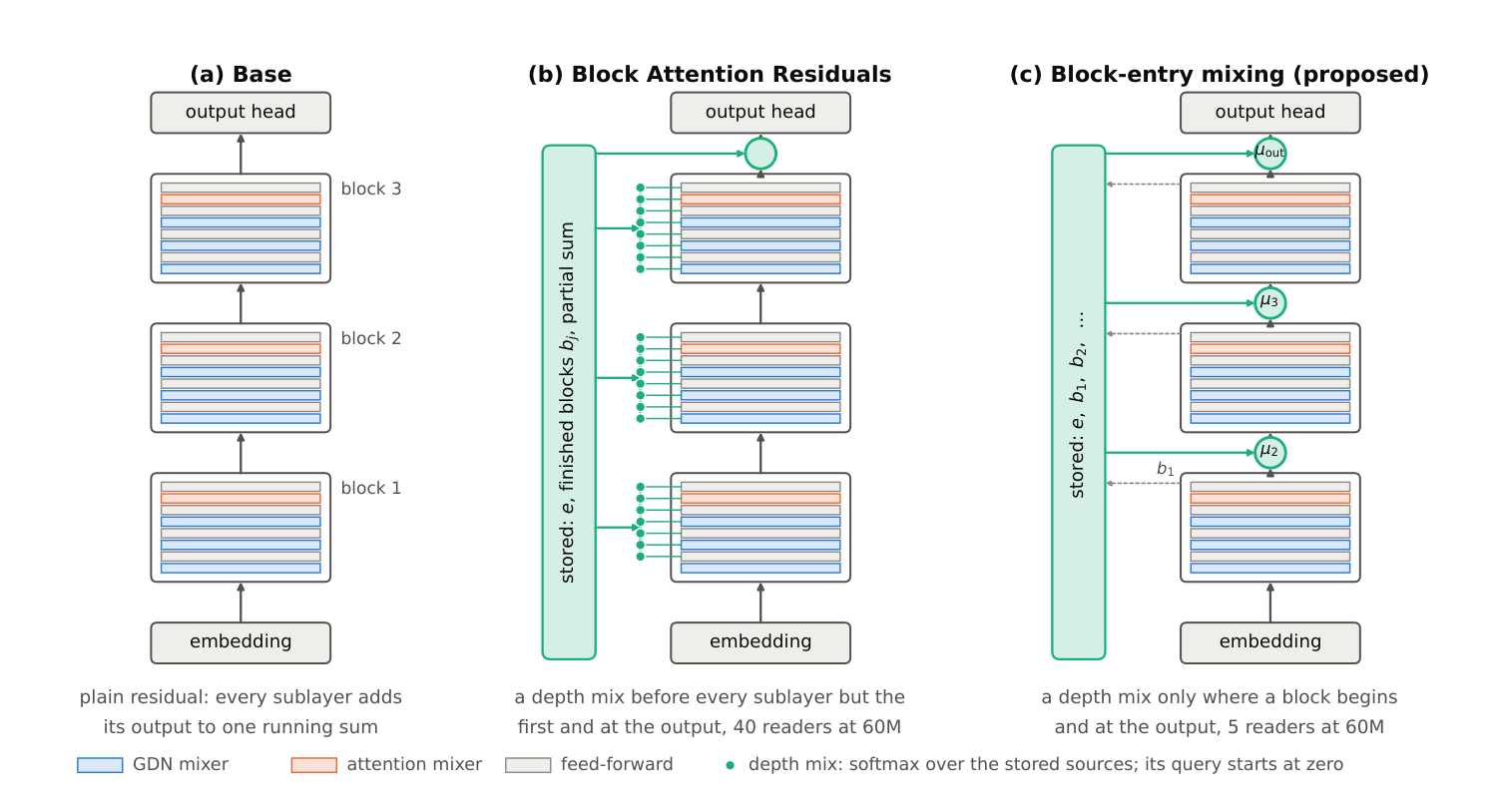
(b) reads before every sublayer but the first, and at the output: 40 readers at 60M. (c) reads only where a block begins, and at the output: 5 readers (report Figure 3).
Five readers kept a little over half of the bpb gain and all of the 16-key retrieval gain at 8k, over two seeds. In the final three-seed set, block-entry mixing beats the base on both bpb and retrieval, and it carries most of F’s retrieval gain. It costs 0.046% of the forward FLOPs and made my unfused step about 3% longer.
Two attempts to make the readers smarter failed, in one seed each. A token-dependent query lost on both counts. Eight heads per reader gained a little bpb but cost retrieval, and from then on I stopped accepting that trade anywhere in the model.
Still open: the cost with a fused kernel at a larger size, and whether it hurts field extraction, which one noisy recall set at 200M hints at.
2. Capped RoPE with a NoPE layer

This one started with a weird plot. Beyond the 8k training length, single-needle retrieval was not monotone in length: it was worse at 16k than at 32k. Putting needles at fixed distances showed a wave with a period of about 20,000 tokens.
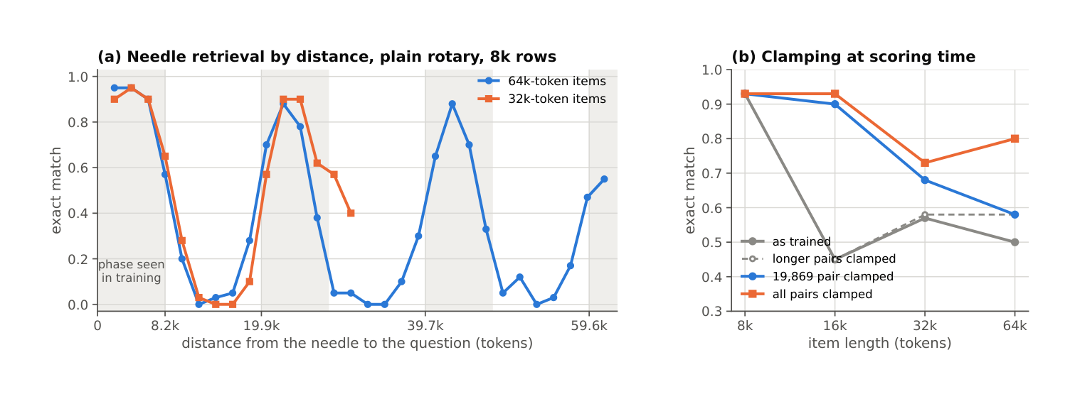
(a) Retrieval follows the phase of one rotary pair. Shaded: the phases training ever showed. (b) Clamping just that pair at scoring time recovers 16k (report Figure 6).
My attention layers use rotary position embeddings (RoPE, from Jianlin Su et al.), and one rotary pair has a wavelength of 19,869 tokens. 8k-token training sequences only ever cover 41% of its cycle. Past that, it produces phases the model never saw. In the one 60M model I traced this in, clamping just that pair’s distance at scoring time, with no training, doubled single-needle retrieval at 16k.
ReRoPE, also from Jianlin Su, treats every distance beyond a fixed cap as the cap, at inference. What I tried is the same cap, C = 2,048, in training as well as at inference. Su also tried training with ReRoPE from the start and reported no length extrapolation. Dropping positions everywhere (NoPE) also avoids unseen phases, but it cost bpb at 8k in one seed. I only ever ran C = 2,048.
The intuition is that exact positions matter only nearby: a key 10,000 tokens back and one 10,001 back mean the same thing to the query. Peter Shaw et al. (2018) capped relative distances in training for the same reason, with learned position embeddings.
This matches Su’s report. With the cap alone, in one seed trained with plain softmax, needle accuracy dropped to 0.22 at 64k and recovered to 0.77 with a scale factor added at inference. So I paired the cap with Scalable-Softmax (Ken M. Nakanishi, 2025), which builds that scale in. Llama 4 scales attention for the same reason. With Scalable-Softmax, over three seeds, the cap left bpb level with plain RoPE, within the seed noise, and kept needle retrieval much steadier beyond 8k. The cap adds no FLOPs.
One attention layer is left without positions, as in Su’s HWFA, Cohere’s RNoPE and Llama 4’s iRoPE. Putting NoPE only in the deepest of the five attention layers (4 capped, 1 NoPE) instead of the two deepest (3 capped, 2 NoPE) added about 0.09 multi-key retrieval in two seeds. That evidence is thin.
Still open: whether the NoPE layer’s gain comes from within the cap or beyond it, and whether NoPE makes generations end less reliably after post-training, as the Qwen team reports for a NoPE variant of its GDN hybrid, Qwen3.8-Next.
3. Separate write and read mixes for GDN

Block-entry mixing already keeps a few depth sources around: the embedding and each block’s output. My hunch was that keys written from shallower inputs stay closer to the token’s identity, which is what a lookup needs.
My first idea was to let a GDN layer read the state of the layer below. That needs a new kernel and roughly doubles the GDN cost. The cheap version: compute the inputs a GDN layer writes with (k, v, β, α) from their own softmax mix of those stored sources. I call it the write mix.
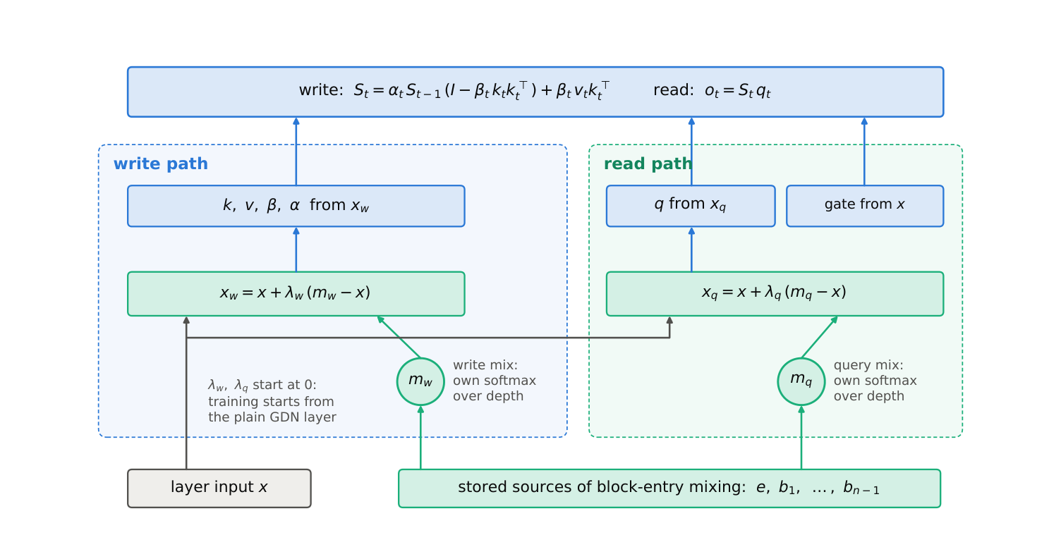
The write path and the query each read their own mix of the stored sources. Both blends start at zero, so training starts from the plain layer (report Figure 7).
The write mix lowered bpb beyond the seed noise, but retrieval dipped, within the noise: the same pattern as the eight-head reader. My guess was that better associations got written but the query could not find them. So the query got its own mix too, the query mix. That kept the bpb gain and brought retrieval back to the no-mix level. In the final three-seed set, though, removing the mixes costs bpb only within the noise.
At 200M, F’s two seeds are further apart on retrieval than F is from its version without the mixes. So whether the mixes cost retrieval at 200M is open.
The mixes are 0.26% of the forward FLOPs, but on unfused code they added 13% to 18% to the step. A fused kernel took the write mix to about 3%, timed in separate jobs, so roughly. The math is light, so most of the overhead is probably the cost of running small separate kernels.
At 200M I also ran three variants that feed the mix to different GDN inputs, one seed each. Mixing only the value, with the keys left on the layer’s own input, still lost retrieval beyond the noise at about half of the ten length and key-count settings, so colliding keys may not be the whole story. But one seed decides nothing. Their second seeds were running or queued when I wrote this, and the results will go into a later version of the report.
4. Grid KV sharing

In GQA, every head in a group uses exactly the same key. Can I keep the cache and still give the heads more distinct keys?
Put the query heads on a grid. Cache one part per row and one per column, each half a head wide. Head (i, j) joins row i’s part and column j’s part into its key, and its value the same way. Then r + c cached parts give r × c distinct keys: at the cache of n KV heads, an n × n grid gives n² distinct keys where GQA gives n.
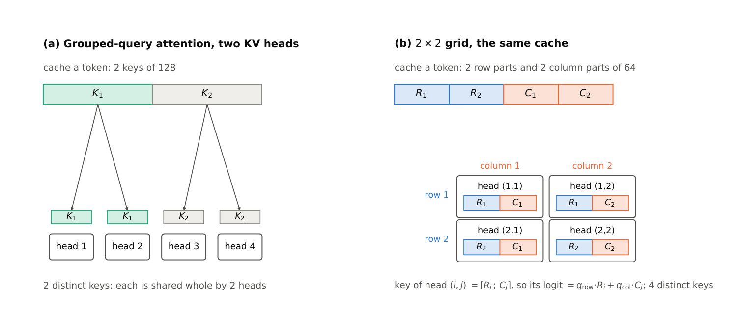
Same cache. GQA with two key–value (KV) heads gives 2 distinct keys, each shared whole by 2 heads. A 2 × 2 grid gives 4, shared in halves (report Figure 9).
Parameters, cache and attention arithmetic stay the same, and on average two heads share as much of their keys as in GQA. What changes is the pattern of sharing. And since a head’s score is a row score plus a column score, its attention is the product of a row pattern and a column pattern: it attends where both match. That last part is my interpretation, not checked yet.
Grid KV came to me after F’s composition was fixed. Folding it in would have meant rerunning the ablation set, which I had neither the time nor the compute for, so I tested it on its own.
At 60M there are only four query heads, and with a 2 × 2 grid against two KV heads the three seeds disagreed on which was better.
At 200M, with eight query heads, a 2 × 2 grid with two heads at each grid position against two KV heads at the same cache had lower bpb in both seeds, by an amount inside the spread of the 200M seeds. Retrieval read lower, within the noise. Most of that gap comes from one of the grid’s two seeds. In short: same cost, more distinct keys, no bpb loss, and no retrieval gain I can separate from noise.
The second 200M pair is a negative result. It put a 2 × 4 grid with the cache of three KV heads (eight distinct keys) against four KV heads (four keys and a third more cache). The grid’s bpb was higher in both seeds, inside the spread. Its 16-key retrieval at 8k, 16k and 32k fell below that of four KV heads, beyond the noise at each of those lengths. Four KV heads also scored higher on FDA, a field-extraction set, in both seeds. And four KV heads beat two on bpb in both seeds, outside the spread. The grid changes how heads share the cache but doesn’t make up for a smaller one. With a quarter less cache it trails four KV heads, most on multi-key retrieval.
Why keep it? It costs nothing to swap in: same parameters, cache and attention FLOPs as GQA. And my runs sit where the gap is smallest: every equal-cache run had 4 keys against 2. In a common large-model setup, 32 to 64 query heads on 8 KV heads’ worth of cache, a grid gives every head its own key where GQA gives 8. That regime is untested.
The closest earlier work I found afterwards is Kronecker product attention (Bahareh Nikpour et al., 2026), which also puts the heads on a grid with one cached factor per row and one per column, and multiplies the two where the grid joins them. Product key memory (Guillaume Lample et al., 2019) uses the same counting, r + c sub-keys joined into r × c keys, for a learned memory table read by top-k.
TST and tied embeddings
Two published methods made it into F. The first is token-superposition training (TST), from Bowen Peng, Théo Gigant and Jeffrey Quesnelle (2026). For the first quarter of training, TST feeds the model bags of 4 averaged token embeddings and has it predict the next bag, so it sees 1.75 times the text for the same compute. In my hybrid the gain was small: about 0.25% bpb on the base, and 0.78% on the model with block-entry mixing (measured against controls from an older version of my code). Most of it lands on rare tokens.
The second is tied embeddings (Ofir Press and Lior Wolf, 2017; Hakan Inan et al., 2017), one matrix for the input embedding and the output head. To keep the comparison fair, I widened the feed-forward layers so that the trunk grew by about the share of parameters that tying frees at the planned 3.8B size, about 5%. With that, tied embeddings lowered bpb beyond the seed noise over two seeds.
Inside F, removing either one made in-context copying (repeating a random token sequence the model has just read) worse, removing tying most of all, over three seeds each. I ran no noise test on the copying measure, so treat this as a direction. Removing TST also costs bpb beyond the seed noise.
Results
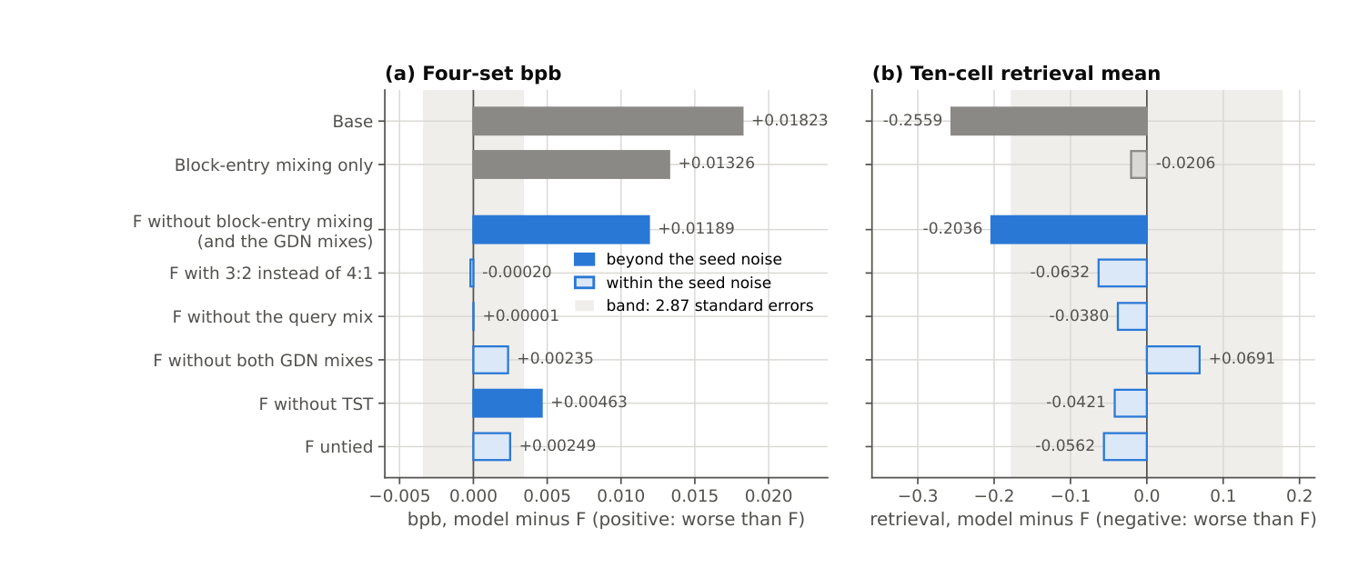
Each model’s difference from F, three seeds per model. Filled bars are beyond the seed noise. The band is 2.87 standard errors (report Figure 11).
Leaving out block-entry mixing (which takes the GDN mixes with it) or TST costs bpb beyond the seed noise, and block-entry mixing also carries the retrieval gain. The other pieces stay within the noise, which with three seeds is not the same as no effect.
At 200M, F has the lowest bpb of any model I trained at that size, over two seeds. Its retrieval moved more between its seeds than between models.
Trained longer at 60M, F kept a lower bpb than the base and than block-entry mixing alone at equal compute, at 1, 2 and 4 times the base’s training budget, by a smaller margin than in the short runs. That is one seed per point.
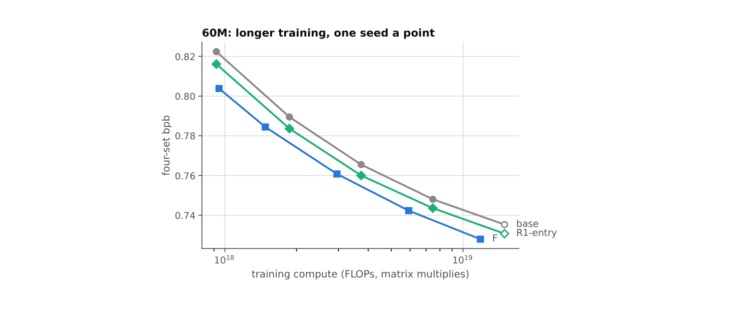
bpb against training compute at 60M, one seed per point. R1-entry in the figure is block-entry mixing (report Figure 13).
For F, half the standard learning rate gave the best bpb, but only within the seed noise of the standard rate. A run at a quarter of the standard rate was queued when I wrote this.
Limitations
- Everything is at 60M and 200M, with three seeds per model in the final 60M set and one or two elsewhere.
- Retrieval is noisy: at 60M a difference must exceed about 0.2 in exact-match accuracy to stand out at two seeds, and at 200M the spread is 1.6 times larger. Most retrieval differences here are directions, not results.
- The retrieval probes are synthetic lookups scored by exact match.
- Step times come from my own compiled but unfused code. Only the block-entry reads and the write mix have fused-kernel measurements, and neither was timed against the base in the same job.
- Almost every run uses Scalable-Softmax, the base included. Apart from the plain-softmax comparisons in the RoPE work, I did not test whether the results hold without it.
Links
- Full report (PDF): github.com/numberingai/gdn-hybrid-architecture-ideas. An arXiv version will follow.
- Code: with the next version of the report, once the remaining runs finish.